Chapter 4 Accounting for Regulations
So far, we have explored various ways to map the distribution of restaurants in San Francisco. Studies have consistently found that restaurants, and other organizational resources like police stations, schools, childcare centers, banks, and parks, are unevenly distributed across neighborhoods by race and class in the US. Surely, race and class are important determinants of the distribution of resources. For example, white and more affluent neighborhoods have more private childcare centers, traditional financial services, “high-end” restaurants while racial minority and poorer neighborhoods have more public childcare centers, alternative financial services, and “unhealthy” restaurants. We can explore these relationships using the aggregated demographic data merged with the POI data, which we’ve discussed so far.
However, the distribution of organizational resources, and more broadly, the built environment is heavily shaped by regulations. Particularly, local zoning laws have tremendous impact on what gets or doesn’t get built in the neighborhood.
In the following, we will discuss how “community benefit districts (CBDs)”, also known as “business improvement districts (BIDs), may have a spatial relationship with the distribution of restaurants in San Francisco. In San Francisco, CBDs are designated based on a private-public partnership to fund improvements and get customized support for commercial and mixed-use corridors in select neighborhoods.
# Import the cbds data
sfzone <- st_read("data/bid_cbd.geojson") %>%
  dplyr::select(community_benefit_district, contract_duration, established, geometry)
## Reading layer `bid_cbd' from data source
## `/Users/hesuyoon/Documents/ENSAE-CREST/Teaching/Advanced_Method/soc-gis-tutorial/data/bid_cbd.geojson'
## using driver `GeoJSON'
## Simple feature collection with 16 features and 12 fields
## Geometry type: MULTIPOLYGON
## Dimension: XY
## Bounding box: xmin: -122.4653 ymin: 37.71984 xmax: -122.3881 ymax: 37.80862
## Geodetic CRS: WGS 84head(sfzone, 3)## Simple feature collection with 3 features and 3 fields
## Geometry type: MULTIPOLYGON
## Dimension: XY
## Bounding box: xmin: -122.4653 ymin: 37.71984 xmax: -122.3997 ymax: 37.78026
## Geodetic CRS: WGS 84
## community_benefit_district contract_duration established geometry
## 1 SoMa West 15 years 2019 MULTIPOLYGON (((-122.4178 3...
## 2 Excelsior 10 years 2023 MULTIPOLYGON (((-122.4385 3...
## 3 Ocean Avenue 15 years 2010 MULTIPOLYGON (((-122.4653 3...# Check the boundaries
ggplot() +
geom_sf(data = sfnh, fill = NA, color = "black", size = 0.2) +
geom_sf(data = sfzone,
aes(fill = community_benefit_district),
color = "white", size = 0.02) +
theme_void() +
labs(title = "Community Benefit Districts in San Francisco")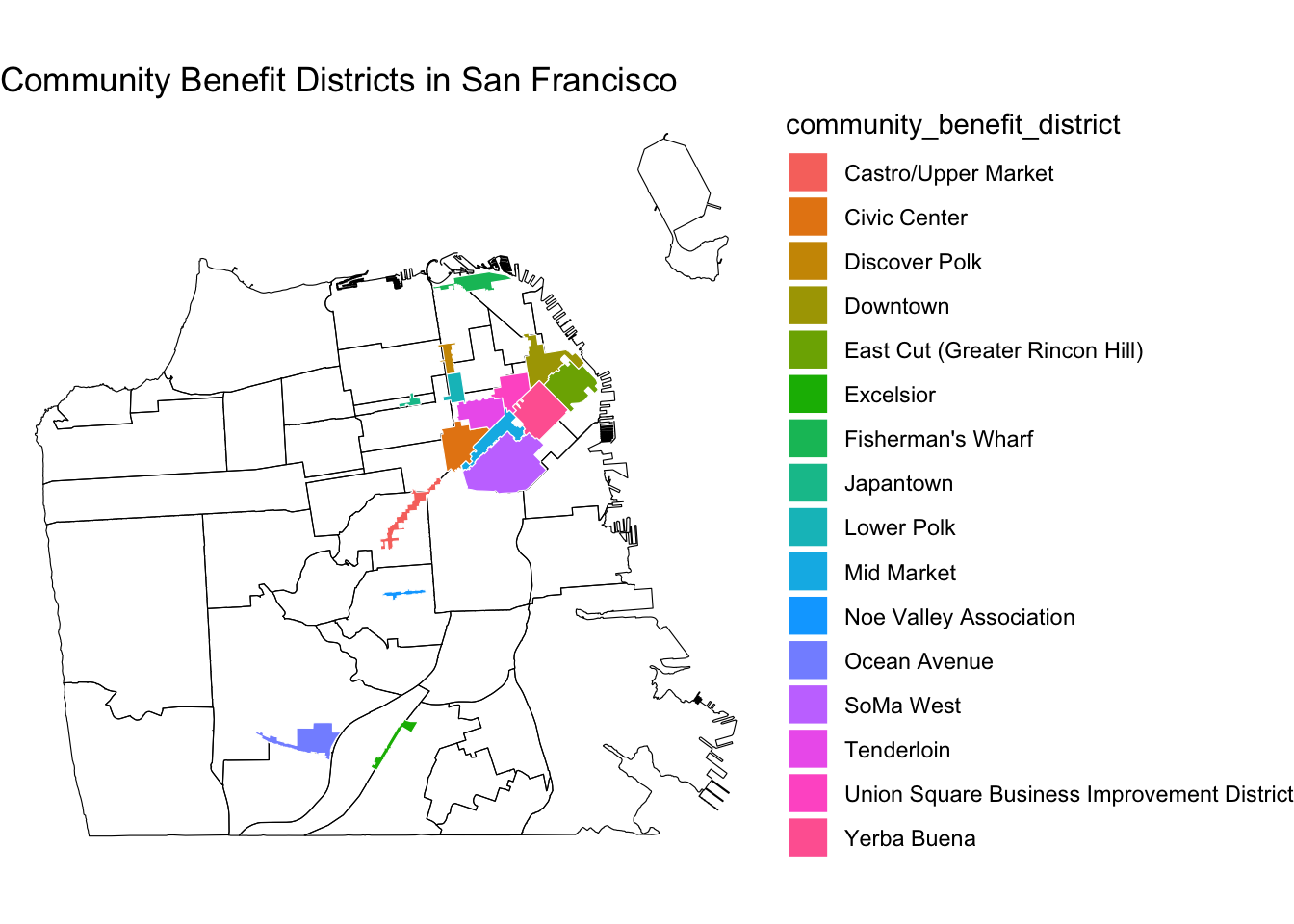
Recollect how restaurants were distributed in San Francisco. We can, for instance, ask if a neighborhood is within or close to BIDs, they are likely to have more businesses. If this was the case, such a spatial proximity could be an important factor in estimating the relationship between a neighborhood and the number of businesses. Below, we will learn how to create a spatial variable at the neighborhood-level, indicating 1) whether the neighborhood intersects with BIDs (binary), as well as 2) its nearest or average distance to BIDs (continuous).
4.1 Spatial functions
First, let’s determine whether a neighborhood boundary intersects with BIDs. We can use st_intersects function to create a list of neighborhoods and its intersecting BIDs.
# Find out if neighborhoods intersect with any BIDs
intersections <- st_intersects(biz_colors, sfzone)

print(intersections)
## Sparse geometry binary predicate list of length 41, where the predicate was
## `intersects'
## first 10 elements:
## 1: 12, 13, 15
## 2: 3
## 3: (empty)
## 4: (empty)
## 5: 1, 6, 9, 11, 13, 14
## 6: (empty)
## 7: (empty)
## 8: (empty)
## 9: (empty)
## 10: (empty)# Create a new binary variable indicating whether a neighborhood intersects with any BIDs
biz_colors$intersects_cbd <- sapply(intersections,
function(x) ifelse(length(x) > 0, 1, 0))
head(biz_colors, 3)## Simple feature collection with 3 features and 3 fields
## Geometry type: MULTIPOLYGON
## Dimension: XY
## Bounding box: xmin: -122.4761 ymin: 37.70833 xmax: -122.3983 ymax: 37.79037
## Geodetic CRS: WGS 84
## nhood n_rst geometry intersects_cbd
## 1 Western Addition 45 MULTIPOLYGON (((-122.4214 3... 1
## 2 West of Twin Peaks 74 MULTIPOLYGON (((-122.461 37... 1
## 3 Visitacion Valley 6 MULTIPOLYGON (((-122.4039 3... 0Here, we can see that a new “intersects_cbd” column was created and added to the sf object, biz_colors.
The second solution requires calculating distance. What is the nearest or average distance to BIDs for a given neighborhood? We use the centroids of polygons for distance calculations.
# Create centroids for both neighborhood polygons and community benefit district polygons
nh_centroids <- st_centroid(sfnh)
bids_centroids <- st_centroid(sfzone)
# Compute pairwise distances (matrix form)
distances <- st_distance(nh_centroids, bids_centroids)
# Convert to a data frame for easier manipulation
distance_df <- as.data.frame(as.matrix(distances))
head(distance_df, 3)## V1 V2 V3 V4 V5 V6 V7
## 1 2113.160 [m] 6330.618 [m] 6579.378 [m] 3389.777 [m] 1824.279 [m] 2582.332 [m] 3287.795 [m]
## 2 6240.084 [m] 2536.732 [m] 1253.155 [m] 3041.710 [m] 4212.930 [m] 7469.365 [m] 8281.413 [m]
## 3 6801.452 [m] 2506.258 [m] 4016.806 [m] 4695.895 [m] 6128.807 [m] 7928.812 [m] 8527.637 [m]
## V8 V9 V10 V11 V12 V13
## 1 2949.494 [m] 2134.726 [m] 3076.620 [m] 1737.384 [m] 414.8295 [m] 1096.984 [m]
## 2 8283.973 [m] 7432.754 [m] 8868.106 [m] 6514.740 [m] 6181.4583 [m] 5951.285 [m]
## 3 8917.746 [m] 8312.261 [m] 10461.030 [m] 7383.877 [m] 8271.5464 [m] 7276.509 [m]
## V14 V15 V16
## 1 1442.067 [m] 1130.678 [m] 1497.141 [m]
## 2 6710.372 [m] 6815.890 [m] 7285.227 [m]
## 3 7873.987 [m] 8384.073 [m] 9011.337 [m]# Add meaningful column and row names
colnames(distance_df) <- sfzone$community_benefit_district
rownames(distance_df) <- sfnh$nhood
head(distance_df, 3)## SoMa West Excelsior Ocean Avenue Noe Valley Association
## Western Addition 2113.160 [m] 6330.618 [m] 6579.378 [m] 3389.777 [m]
## West of Twin Peaks 6240.084 [m] 2536.732 [m] 1253.155 [m] 3041.710 [m]
## Visitacion Valley 6801.452 [m] 2506.258 [m] 4016.806 [m] 4695.895 [m]
## Castro/Upper Market Yerba Buena East Cut (Greater Rincon Hill)
## Western Addition 1824.279 [m] 2582.332 [m] 3287.795 [m]
## West of Twin Peaks 4212.930 [m] 7469.365 [m] 8281.413 [m]
## Visitacion Valley 6128.807 [m] 7928.812 [m] 8527.637 [m]
## Downtown Union Square Business Improvement District Fisherman's Wharf
## Western Addition 2949.494 [m] 2134.726 [m] 3076.620 [m]
## West of Twin Peaks 8283.973 [m] 7432.754 [m] 8868.106 [m]
## Visitacion Valley 8917.746 [m] 8312.261 [m] 10461.030 [m]
## Mid Market Japantown Civic Center Tenderloin Lower Polk
## Western Addition 1737.384 [m] 414.8295 [m] 1096.984 [m] 1442.067 [m] 1130.678 [m]
## West of Twin Peaks 6514.740 [m] 6181.4583 [m] 5951.285 [m] 6710.372 [m] 6815.890 [m]
## Visitacion Valley 7383.877 [m] 8271.5464 [m] 7276.509 [m] 7873.987 [m] 8384.073 [m]
## Discover Polk
## Western Addition 1497.141 [m]
## West of Twin Peaks 7285.227 [m]
## Visitacion Valley 9011.337 [m]# Reshape to a long-format for analysis
distance_long <- distance_df %>%
rownames_to_column("Neighborhood") %>% # convert row names into a new column
pivot_longer(
cols = -Neighborhood, # pivot all columns except "Neighborhood"
names_to = "BID", # names of the column will become values in "BID"
values_to = "Distance" # values will go into "Distance" column
)
head(distance_long, 10)## # A tibble: 10 × 3
## Neighborhood BID Distance
## <chr> <chr> [m]
## 1 Western Addition SoMa West 2113.
## 2 Western Addition Excelsior 6331.
## 3 Western Addition Ocean Avenue 6579.
## 4 Western Addition Noe Valley Association 3390.
## 5 Western Addition Castro/Upper Market 1824.
## 6 Western Addition Yerba Buena 2582.
## 7 Western Addition East Cut (Greater Rincon Hill) 3288.
## 8 Western Addition Downtown 2949.
## 9 Western Addition Union Square Business Improvement District 2135.
## 10 Western Addition Fisherman's Wharf 3077.# Identify nearest distance BID
nearest_bid <- distance_long %>%
group_by(Neighborhood) %>%
slice_min(order_by = Distance)
head(nearest_bid, 10)## # A tibble: 10 × 3
## # Groups: Neighborhood [10]
## Neighborhood BID Distance
## <chr> <chr> [m]
## 1 Bayview Hunters Point Excelsior 4284.
## 2 Bernal Heights Noe Valley Association 1890.
## 3 Castro/Upper Market Castro/Upper Market 502.
## 4 Chinatown Downtown 733.
## 5 Excelsior Excelsior 741.
## 6 Financial District/South Beach East Cut (Greater Rincon Hill) 329.
## 7 Glen Park Noe Valley Association 1361.
## 8 Golden Gate Park Castro/Upper Market 4487.
## 9 Haight Ashbury Castro/Upper Market 1221.
## 10 Hayes Valley Civic Center 934.# Join the distance data to the existing neighborhood-level spatial data
biz_colors <- biz_colors %>%
left_join(nearest_bid,
by = c("nhood" = "Neighborhood"))
# Alternatively, you can directly add the distance variable using apply function
biz_colors$min_distance_to_bid <- apply(distances, # use distances matrix
1, # apply to rows
min) # get minimum
head(biz_colors, 3)## Simple feature collection with 3 features and 6 fields
## Geometry type: MULTIPOLYGON
## Dimension: XY
## Bounding box: xmin: -122.4761 ymin: 37.70833 xmax: -122.3983 ymax: 37.79037
## Geodetic CRS: WGS 84
## nhood n_rst intersects_cbd BID Distance
## 1 Western Addition 45 1 Japantown 414.8295 [m]
## 2 West of Twin Peaks 74 1 Ocean Avenue 1253.1553 [m]
## 3 Visitacion Valley 6 0 Excelsior 2506.2580 [m]
## geometry min_distance_to_bid
## 1 MULTIPOLYGON (((-122.4214 3... 414.8295
## 2 MULTIPOLYGON (((-122.461 37... 1253.1553
## 3 MULTIPOLYGON (((-122.4039 3... 2506.2580Instead of just looking at the nearest neighbor, if you want the average of the nearest three or specific number of neighbors, you can specify the number and get the average as well.
# Identify three nearest BIDs
nearest_three_bid <- distance_long %>%
  group_by(Neighborhood) %>%
  slice_min(order_by = Distance,
            n = 3) # the number of nearest neighbors

# Calculate the average distance
avg_distance_to_bids <- nearest_three_bid %>%
  group_by(Neighborhood) %>%
  summarize(avg_distance = mean(Distance, na.rm = TRUE))

# Join the distance data to the existing neighborhood-level spatial data
biz_colors <- biz_colors %>%
  left_join(avg_distance_to_bids,
            by = c("nhood" = "Neighborhood"))

head(biz_colors, 3)
## Simple feature collection with 3 features and 7 fields
## Geometry type: MULTIPOLYGON
## Dimension: XY
## Bounding box: xmin: -122.4761 ymin: 37.70833 xmax: -122.3983 ymax: 37.79037
## Geodetic CRS: WGS 84
## nhood n_rst intersects_cbd BID Distance min_distance_to_bid
## 1 Western Addition 45 1 Japantown 414.8295 [m] 414.8295
## 2 West of Twin Peaks 74 1 Ocean Avenue 1253.1553 [m] 1253.1553
## 3 Visitacion Valley 6 0 Excelsior 2506.2580 [m] 2506.2580
## avg_distance geometry
## 1 880.8306 [m] MULTIPOLYGON (((-122.4214 3...
## 2 2277.1990 [m] MULTIPOLYGON (((-122.461 37...
## 3 3739.6530 [m] MULTIPOLYGON (((-122.4039 3...This type of distance data can be used for network analysis to study urban connectivity, accessibility, and so forth. In network terms, a Neighborhood is ego, and a BID is alter. Distance is edge, connecting ego and alter. Network analysis is beyond the scope of this tutorial, but remember, handling spatial data is a powerful tool that will enable you to conduct advanced statistical analysis.
Now, you have a neighborhood-level data with the number of restaurants (n_rst) as an outcome variable, and three spatial predictors - intersects_cbd, min_distnace_distance_to_bid, and avg_distance_to_bids. You can always merge additional predictors, such as aggregated demographic variables, which we covered in the beginning of the tutorial.
With this neighborhood-level data, you could run a bivariate regression model estimating the relationship between the number of businesses and being in BIDs.
# Run the bivariate ols regression model
model <- lm(n_rst ~ intersects_cbd, data = biz_colors)

# View the summary of the model
summary(model)
##
## Call:
## lm(formula = n_rst ~ intersects_cbd, data = biz_colors)
##
## Residuals:
## Min 1Q Median 3Q Max
## -87.32 -39.77 -19.32 30.23 223.68
##
## Coefficients:
## Estimate Std. Error t value Pr(>|t|)
## (Intercept) 39.77 14.41 2.761 0.00874 **
## intersects_cbd 65.54 21.16 3.097 0.00361 **
## ---
## Signif. codes: 0 '***' 0.001 '**' 0.01 '*' 0.05 '.' 0.1 ' ' 1
##
## Residual standard error: 67.57 on 39 degrees of freedom
## Multiple R-squared: 0.1974, Adjusted R-squared: 0.1768
## F-statistic: 9.594 on 1 and 39 DF, p-value: 0.00361This simple analysis demonstrates that neighborhoods that intersect BIDs, on average, indeed have 65.54 more businesses compared to neighborhoods that do not intersect with BIDs. Such a spatial variable can be included as a main predictor or as a control variable depending on your research question.
CODING EXERCISE
- Create spatial variables between neighborhoods and historic districts
- Import the historic district data.
- Create a binary variable based on whether the neighborhood overlaps with any historic districts.
- Calculate distance of the three nearest historic districts for each neighborhood.
4.2 Constructing Geometry
In the following, we will learn some techniques that enable you to manipulate geometries. Specifically, we will focus on three geometric operations: aggregating polygons, creating a buffer zone, and extracting overlapping areas.
AGGREGATING POLYGONS
In San Francisco, there are 16 BIDs. In the original data, these districts come as separate polygons. However, you could combine them into one polygon.
# Create a simple union
sfzone_union <- st_union(sfzone)

head(sfzone_union, 3)
## Geometry set for 1 feature
## Geometry type: MULTIPOLYGON
## Dimension: XY
## Bounding box: xmin: -122.4653 ymin: 37.71984 xmax: -122.3881 ymax: 37.80862
## Geodetic CRS: WGS 84## MULTIPOLYGON (((-122.4304 37.78693, -122.4305 3...# Display the new polygon
plot(st_geometry(sfzone_union))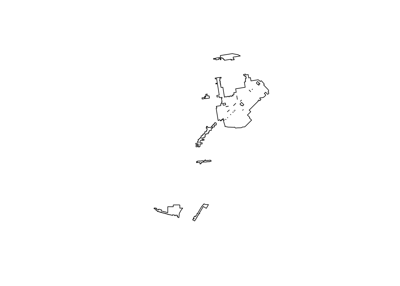
# Compare it with the original BIDs
ggplot() +
  # add neighborhood boundaries
  geom_sf(data = sfnh, fill = "light grey", color = "white", size = 0.3) +
  # add BID boundaries
  geom_sf(data = sfzone, fill = "light blue", color = "black", size = 0.3)+
  # add combined BIDs
  geom_sf(data = sfzone_union, fill = NA, color = "red", size = 1.5) +
  theme_void()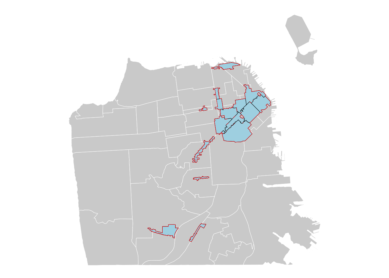
Taking a step further from a simple aggregation, you can create combined polygons based on a grouping variable. For example, we know when each BID was established. We can divide BIDs into those established before/after 2010, and create two BID polygons that are new vs. old.
# Add a column to classify BIDs
sfzone <- sfzone %>%
  mutate(bid_type = ifelse(established > 2010, "New", "Old"))

# Aggregate polygons by BID_Type
sfzone_by_type <- sfzone %>%
  group_by(bid_type) %>%
  summarize(geometry = st_union(geometry), .groups = "drop")

head(sfzone_by_type, 3)
## Simple feature collection with 2 features and 1 field
## Geometry type: MULTIPOLYGON
## Dimension: XY
## Bounding box: xmin: -122.4653 ymin: 37.71984 xmax: -122.3881 ymax: 37.80862
## Geodetic CRS: WGS 84
## # A tibble: 2 × 2
## bid_type geometry
## <chr> <MULTIPOLYGON [°]>
## 1 New (((-122.4021 37.78872, -122.4014 37.78926, -122.4008 37.78882, -122.4003 37.78844…
## 2 Old (((-122.436 37.75922, -122.4361 37.76054, -122.436 37.76054, -122.4356 37.76056, …# Visualize
ggplot() +
# add neighborhood boundaries
geom_sf(data = sfnh, fill = "light grey", color = "white", size = 0.3) +
# aggregated BIDs by type
geom_sf(data = sfzone_by_type,
aes(fill = bid_type),
color = "black", size = 0.3) +
theme_void() +
labs(fill = "BID Type")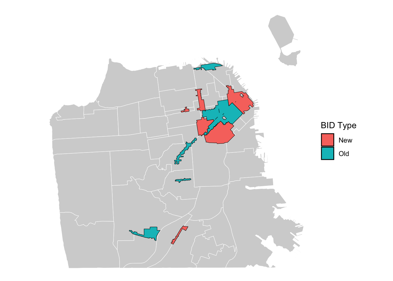
BUILDING BUFFER ZONES
The function st_buffer() allows to construct buffer zones. It takes in a buffer distance and geometry type and outputs a polygon with a boundary the buffer distance away from the input geometry. Buffer zones are useful to think about spatial spill over effects, for example. Take the case of BIDs. Since BIDs help improve the commercial corridors, you can expect that areas (or businesses) located within BIDs might experience positive economic impact. Moreover, those that are not within, but in the vicinity of BIDs may also receive positive impacts by the function of proximity. Such a process can be conceptualized as spatial spill over effects. To address this issue, you could create buffers.
# Create a buffer around the BID boundaries (e.g., 200 meters)
bid_buffer <- st_buffer(sfzone, dist = 200)

head(bid_buffer, 3)
## Simple feature collection with 3 features and 4 fields
## Geometry type: POLYGON
## Dimension: XY
## Bounding box: xmin: -122.4676 ymin: 37.71796 xmax: -122.3973 ymax: 37.78221
## Geodetic CRS: WGS 84
## community_benefit_district contract_duration established geometry
## 1 SoMa West 15 years 2019 POLYGON ((-122.3984 37.7767...
## 2 Excelsior 10 years 2023 POLYGON ((-122.4392 37.7183...
## 3 Ocean Avenue 15 years 2010 POLYGON ((-122.4464 37.7209...
## bid_type
## 1 New
## 2 New
## 3 Old# Exclude the BID area from the buffer
surrounding_buffer <- st_difference(bid_buffer, sfzone_union)
plot(st_geometry(bid_buffer))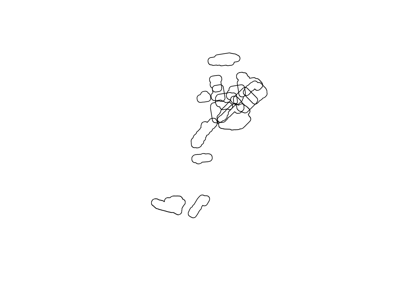
plot(st_geometry(surrounding_buffer))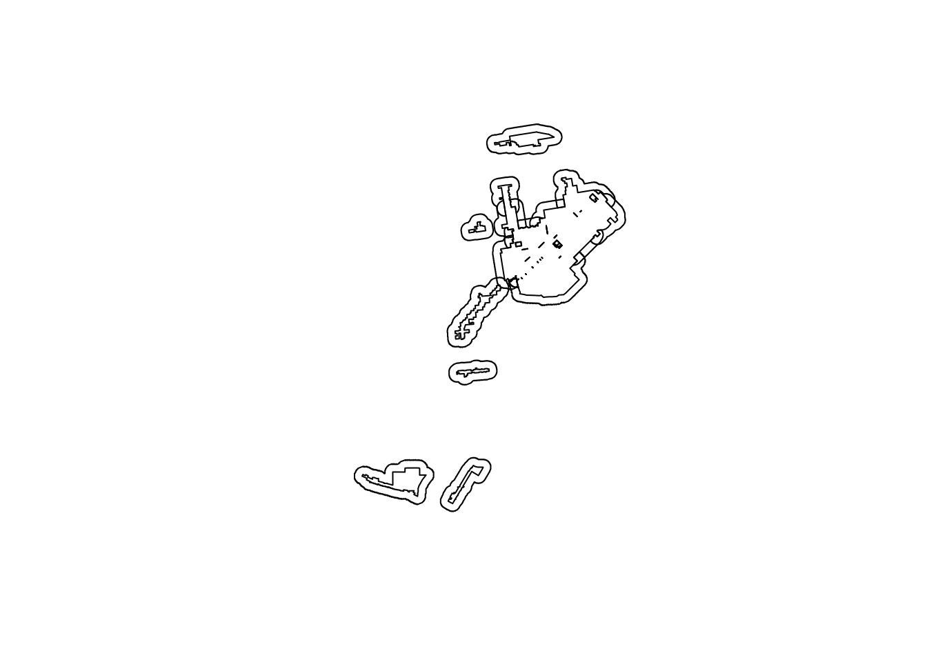
# Create a plot displaying buffer zones around neighborhoods
ggplot() +
  # add neighborhoods
  geom_sf(data = sfnh, fill = "lightgray", color = "white", size = 0.2) +
  # add buffer zones
  geom_sf(data = bid_buffer, fill = "blue", alpha = 0.1, color = "blue", size = 0.5) +
  # add BID boundaries
  geom_sf(data = sfzone, fill = NA, color = "red", size = 1) +
  # style the map
  theme_void()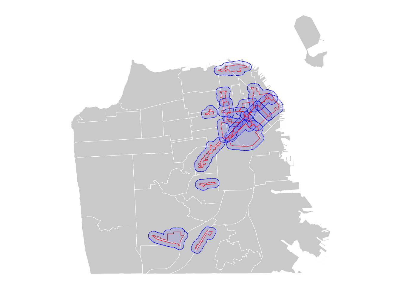
INTERSECTING POLYGONS
We can also extract overlapping areas of two polygons and create a new geometry. Let’s say if you’re interested in focusing on areas that are central in San Francisco.
# Create a central circle
circle <- sftrt %>%
  st_union() %>%
  st_centroid() %>%
  st_buffer(2000)

# Display the circle
ggplot() +
  # add neighborhoods
  geom_sf(data = sftrt, fill = "lightgray", color = "white", size = 0.2) +
  # add a circle
  geom_sf(data = circle, fill = "red", alpha = 0.5, color = "green", size = 0.5) +
  # style the map
theme_void() 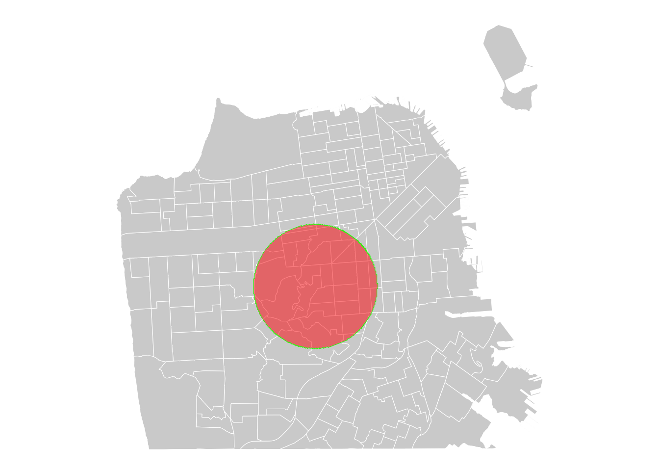
# Get the overlapping area
sf_circle <- st_intersection(x = sftrt, y = circle)
## Warning: attribute variables are assumed to be spatially constant throughout all geometriesplot(st_geometry(sf_circle), border = "black")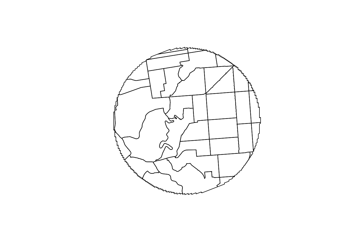
# Highlight the central area in SF
ggplot() +
  # add neighborhoods
  geom_sf(data = sftrt, fill = "lightgray", color = "white", size = 0.2) +
  # add a circle
  geom_sf(data = sf_circle, fill = "red", alpha = 0.5, color = "green", size = 0.5) +
  # style the map
theme_void() 
By the same token, you can identify and map areas that intersect with both BIDs and historic districts in SF.
# Import historic district data
historic <- st_read("data/historic_district.geojson")
## Reading layer `historic_district' from data source
## `/Users/hesuyoon/Documents/ENSAE-CREST/Teaching/Advanced_Method/soc-gis-tutorial/data/historic_district.geojson'
## using driver `GeoJSON'
## Simple feature collection with 191 features and 12 fields
## Geometry type: MULTIPOLYGON
## Dimension: XY
## Bounding box: xmin: -122.5111 ymin: 37.70815 xmax: -122.3571 ymax: 37.8333
## Geodetic CRS: WGS 84# Get intersecting polygons
bid_historic <- st_intersection(x = historic, y = sfzone)
# Visualize the overlapping areas
ggplot() +
# add neighborhoods
geom_sf(data = sfnh, fill = "lightgray", color = "white", size = 0.2) +
# add BIDs
geom_sf(data = sfzone, fill = NA, alpha = 0.5, color = "red", size = 0.5) +
# add historic districts
geom_sf(data = historic, fill = NA, alpha = 0.5, color = "blue", size = 0.5) +
# add the overlapping areas
geom_sf(data = bid_historic, fill = "green", alpha = 0.5, color = NA) +
# style the map
theme_void() 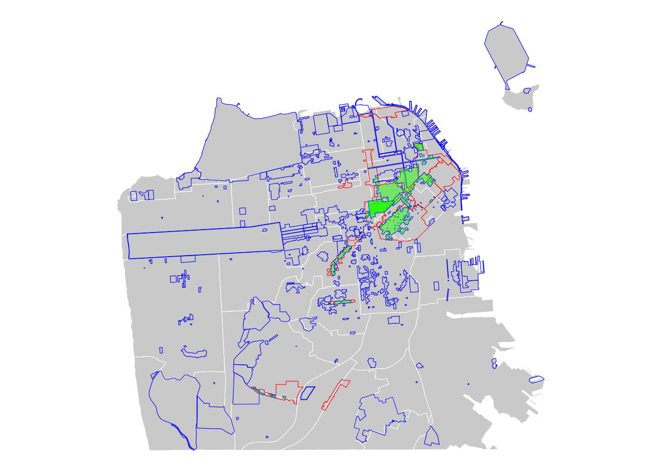
LEARN MORE
Remember three different forms of vector data? We have discussed polygons, points.. and what’s left? Lines. Lines are useful when you are interested in exploring and visualizing transportation networks, mobility patterns, connectivity, and so forth. We won’t cover much details about the line formatted data, but will provide a short example of mapping lines.
During COVID, San Francisco city government launched the Slow Street Program to help maintain social distance requirements for users on the streets. Slow Streets utilize temporary tools like cones and signage to divert traffic and remind vehicles to maintain a safe speed to accommodate for pedestrians and bicyclists who may be traveling to make essential trips. After COVID, this program continued as part of a connected, citywide Active Transportation Network, designed to eliminate deaths and severe injuries related to transportation, and encourage more people to choose low-carbon ways to travel for their daily trips.
# Import slow street data (lines)
slowst <- st_read("data/slow_st.geojson")
## Reading layer `slow_st' from data source
## `/Users/hesuyoon/Documents/ENSAE-CREST/Teaching/Advanced_Method/soc-gis-tutorial/data/slow_st.geojson'
## using driver `GeoJSON'
## Simple feature collection with 240 features and 22 fields
## Geometry type: LINESTRING
## Dimension: XY
## Bounding box: xmin: -122.5056 ymin: 37.71392 xmax: -122.3902 ymax: 37.7905
## Geodetic CRS: WGS 84ggplot() +
geom_sf(data = sfnh, fill = "lightgrey", color = "white", size = 0.2) +
geom_sf(data = slowst,
color = "blue",
size = 50,
linetype = "solid") + # options: dashed, dotted, etc
theme_void()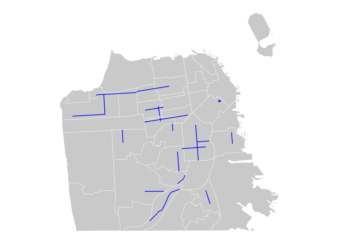
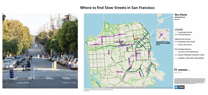
Source: SFMTA (Accessed 2024)
THINK AND SHARE
What other regulations, including but not limited to zoning, can you think of that have meaningful impact on spatial organization of people and the built environment?
For example, scholars have examined the relationship between historic districts and neighborhood change (McCabe and Ellen, 2016) and the impact of BIDs on property values (Ellen et al, 2007).
- What are their research questions?
- How did these authors build and analyze their data?
- What are the key findings?
What kind of research questions can you ask about the impact of zoning? Discuss the potential predictors (x) or outcomes (y).